
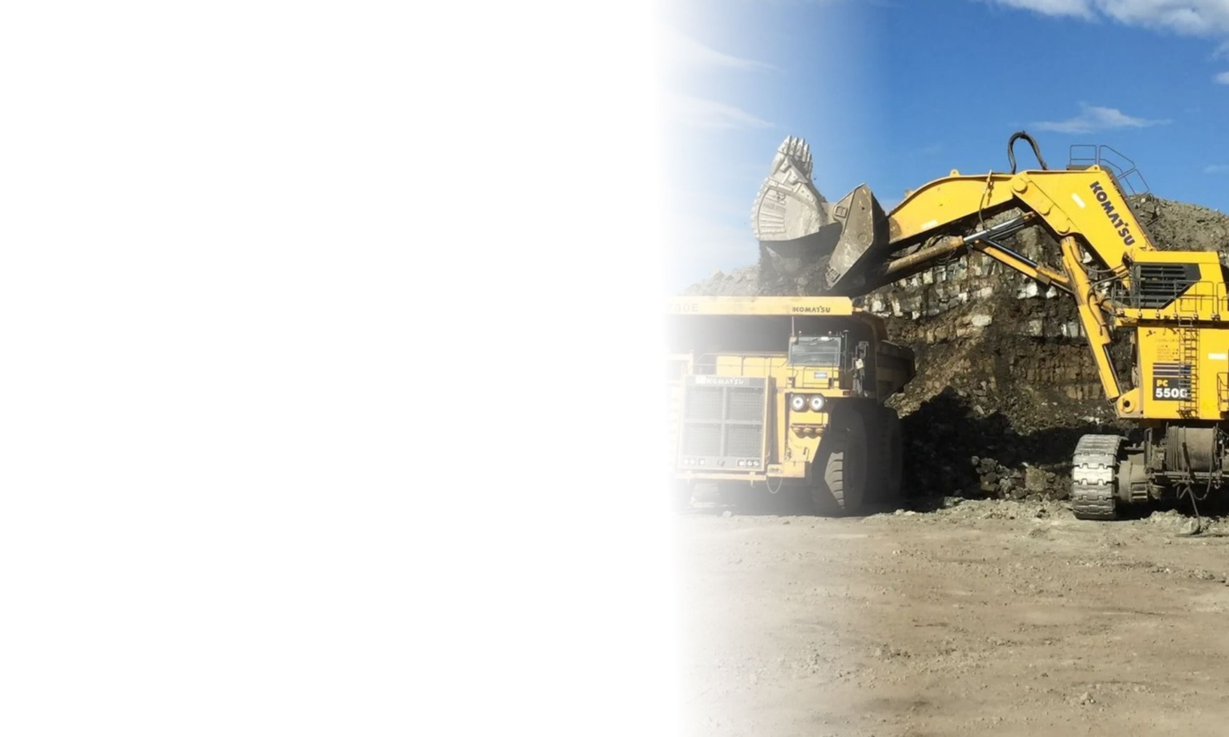
BUILT FOR THE DEMANDS OF HEAVY HAULAGE
Stronger haul roads.
Better mining roads.
Put road performance at the center of your operation. Explore Claycrete II™ soil stabilization for haul roads and mining roads—and model the cost of rolling resistance across your fleet.
Road strength
Start with site-specific soil testing
Fleet economics
Explore rolling-resistance costs
Practical planning
Build a treatment plan for your site
THE ROAD BENEATH YOUR OPERATION
Haul road stabilization starts with the ground.
Haul roads and mining roads carry repeated heavy loads, day after day. Their condition influences the work required to move a truck, the demand for road maintenance, and the management of dust and water.
Claycrete II™ is a soil stabilizer for suitable clay-bearing materials. A successful mining road stabilization program begins with material testing, road design, drainage, and a controlled construction process.
Build for repeated heavy loads
Evaluate road strength and treatment suitability against the loading and operating conditions of your haul fleet.
01
Plan for dust and maintenance
Assess watering, grading, and surface performance as part of a site-specific haul road maintenance strategy.
02
Make the economics visible
Compare existing and improved road-strength scenarios using the rolling-resistance calculator below.
03
Haul Road Savings Calculator
What could a stronger mining road mean for your operation? Select your haul truck, compare road strength, and enter your haul cycle to estimate the change in rolling-resistance energy cost.
Loaded + empty return • annual fleet estimate
Annual modeled saving
Rolling-resistance energy cost only
Annual modeled cost comparison
Planning estimate based on the supplied workbook. This is not a total fuel bill or a guaranteed saving. Treatment and implementation costs are excluded.
The detail, when you need it.
Review or customize the assumptions without crowding the main calculator.
Advanced assumptions & equipment settings
Defaults reproduce the spreadsheet. Selecting a truck resets its mass, wheel load, contact radius, and empty-load factors; it keeps your road and fleet inputs.
Road model
The workbook saves k = 15 for both scenarios. A workbook note mentions k = 20 for Claycrete-treated soils; change it only when appropriate for your site.
Selected equipment
Empty return assumptions
The workbook assumes the empty contact radius and beta equal the loaded values. Here you can override either. The two empty-load factors default to 0.42.
Detailed calculation breakdown
Results below use the most recently calculated inputs.
| Metric | Loaded existing | Loaded improved | Return existing | Return improved | Units |
|---|
| Metric | Existing | Improved / saving |
|---|
Formulas, source notes & model limitations
How the calculation works
- Modulus: E (MPa) = CBR × k; E (Pa) = E (MPa) × 1,000,000.
- Deflection: δ = wheel load ÷ (π × contact radius × E in Pa).
- Rolling resistance: RR = α × δ + β. Multiply by 100 to show a percentage.
- Tractive force: F = RR × vehicle mass × gravity.
- Journey energy: MJ = F × journey distance ÷ 1,000,000.
- Fuel equivalent: liters = MJ ÷ diesel energy density. Journey cost = liters × diesel price.
- Calculate loaded and empty journeys separately. Empty mass and wheel load use their respective factors.
- Annual cycles = cycles per truck per day × fleet size × operating days.
- Annual saving = (existing cycle cost − improved cycle cost) × annual cycles.
What this estimate includes
Only the modeled energy cost attributed to rolling resistance on the selected journey segments. Both road scenarios use the same operating schedule, fuel price, and truck settings. Each daily cycle includes one loaded trip and, when selected, one empty return.
What it does not include
Engine or drivetrain efficiency, gradient, aerodynamic drag, acceleration, idling, auxiliaries, speed or cycle-time changes. The spreadsheet divides mechanical energy directly by diesel energy content; its liters are therefore fuel-energy equivalents, not a prediction of actual fuel consumption. No efficiency multiplier has been added.
Water spraying, tire wear, maintenance, productivity, emissions, treatment cost, payback, and net return on investment are not quantified by the source formulas and are excluded. The workbook’s narrative tire-saving range is not added to the result.
Workbook audit decisions
- All three visible sheets—Calculator, README, and Haul Truck Library—and the hidden Formula_Audit sheet were reviewed.
- The headline uses the complete cycle (Calculator rows 104–121), rather than the earlier loaded-only headline cards.
- All nine truck presets are copied from the supplied library. These are workbook reference values, not independently verified manufacturer specifications.
- CBR is not capped at 100: the workbook itself uses an improved CBR of 200, despite its conflicting validation rule.
- Tire size and pressure are reference information; they do not independently feed the formulas. Contact radius is not recalculated from pressure.
- Negative savings remain visible as a modeled cost increase. Zero trips, distance, or fuel price correctly produce zero applicable costs.
- The saved source uses k = 15 for the improved scenario, despite a note mentioning 20 for treated soil. The calculator preserves 15.
- The source print area ends at row 76, so the return-leg and complete-cycle sections below it can be missed in a printed copy.
Source: Rolling Resistance Reduction - Cost Savings Version 1.01.xlsx. This calculator reproduces its empirical model; site calibration and review are needed before using estimates in a business case. Source workbook copyright notice retained: © 18 June 2026.
Workbook field map & verification
Input-to-cell trace
| Calculator input | Source cell / range | Saved default |
|---|---|---|
| Truck selection | Calculator!H12 | Caterpillar 797F |
| Existing / improved CBR | Calculator!C15 / I15 | 50 / 200 |
| Existing / improved k | Calculator!C16 / I16 | 15 / 15 |
| Wheel load / contact radius / mass | Calculator!C28 / C29 / C32 | Truck-library lookup |
| Alpha / beta | Calculator!C30 / C31 | 80 / 0.01 |
| Gravity | Calculator!C33 | 9.81 m/s² |
| Loaded distance | Calculator!C34 | 5,000 m |
| Diesel energy / price | Calculator!C35 / C36 | 38.6 MJ/L / AUD 1.80 per L |
| Cycles / trucks / days | Calculator!C37:C39 | 12 / 10 / 365 |
| Empty mass / wheel-load factors | Calculator!C79 / C80 | 0.42 / 0.42 |
| Return distance / radius / beta | Calculator!C81 / C84 / C85 | Linked to loaded values |
| Equipment presets | Haul Truck Library!A4:L12 | Nine models |
Default-result reconciliation
| Workbook result | Source cell | AUD |
|---|---|---|
| Loaded annual saving | H48 | 4,101,365.09 |
| Empty-return annual saving | D101 | 723,480.80 |
| Complete-cycle existing annual cost | C110 | 7,410,462.75 |
| Complete-cycle improved annual cost | D110 | 2,585,616.86 |
| Complete-cycle annual saving | D111 | 4,824,845.89 |
The implementation was checked against ten saved workbook results to within AUD 0.000001 or equivalent numeric precision, with all nine presets checked for loaded-plus-return reconciliation. Additional checks cover loaded-only mode, unchanged road strength, negative savings, zero activity, fleet scaling, and invalid inputs.
Interpretation decisions
The README describes editable highlighted cells, truck lookups, and the return-leg extension. Formula_Audit confirms the same energy chain as Calculator. Neither provides an independent physical calibration or a machine-efficiency model. The final workbook note links road roughness to k, but supplies no numerical roughness-to-k function, so no roughness slider or automatic k adjustment is invented.
The source contains no formulas for monetary tire, water, maintenance, or productivity benefits. Those are not added as presumed savings. Client name, prepared-by, and issue-date fields are presentation metadata rather than savings drivers and are omitted from the main view.
The fleet uses one selected model at a time. A mixed fleet should be calculated separately for each model and its actual truck count; annual savings can then be added without counting the same trucks twice.
FROM ASSESSMENT TO APPLICATION
A practical plan for your mining roads.
Match the material, construction method, and performance targets to the site.
01 / ASSESS
Test your road material
Review soil characteristics and existing road strength before selecting treatment parameters.
02 / PLAN
Define the treatment
Discuss traffic loads, drainage, treatment depth, and construction requirements with the project team.
03 / CONSTRUCT
Apply, mix, and compact
Scarify the road, apply Claycrete II™, mix through the material, compact, and trim the surface.
04 / VERIFY
Check site performance
Use agreed site testing and operating observations to assess the finished road against project targets.
HAUL ROAD PLANNING ESSENTIALS
Questions about haul roads & mining roads.
-
Claycrete II™ is offered for haul road stabilization using suitable clay-bearing materials. Soil testing and project assessment are needed to determine whether a particular mining road is a suitable candidate.
-
Deformation under a truck’s tires contributes to the resistance it must overcome. The calculator compares CBR-based road-strength scenarios to model this component of journey energy cost. Actual fuel use also depends on many other operating conditions.
-
It compares rolling-resistance energy costs for the selected truck, road strength, haul distance, diesel price, fleet size, and operating schedule. You can include an empty return journey. It excludes treatment cost and other operating costs; review the detailed assumptions in the calculator.
-
Start with the road location, dimensions, available soil test results, existing surface conditions, haul truck types and loads, traffic schedule, drainage, and maintenance practices. Claycrete Global can discuss the next assessment steps.
TURN THE ESTIMATE INTO A PROJECT CONVERSATION
Let's assess your next haul road.
Bring your calculator assumptions and soil information. Discuss a stabilization approach for the conditions on your site.